Self Organizing Map 에 대해서 알아보겠습니다.
Udemy 의 Deep-Learning-A-to-Z 강의 의 SOM 파트를 수강하고 작성하였습니다.
Self Organizing Map은 줄여서 SOM 이라고 부릅니다.
Unsupervised learning 방법 중 하나이며 Clustering 에 쓰입니다.
Clustering 작업을 수행하는, SOM 보다 조금 단순한 K-mean 알고리즘을 보고 SOM 을 보면 이해가 쉽습니다.
K-mean Cluster
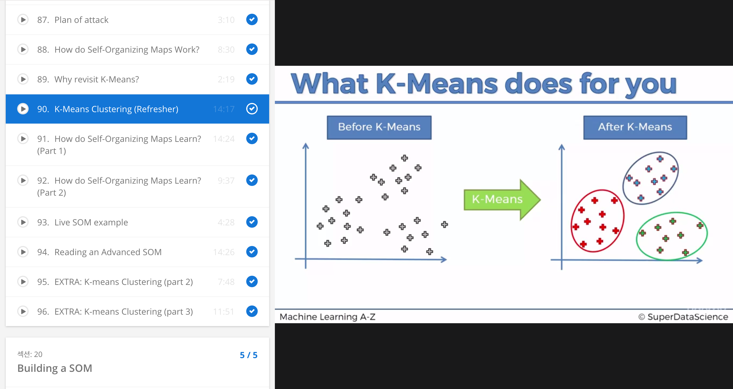
K-mean 의 결과 = Clustering
아래의 그림은 K-mean 알고리즘으로 클러스터링 한 결과를 보여줍니다.
K-mean 의 학습 과정

K-mean 의 학습과정은 단순합니다.
| 과정 | |
|---|---|
| step1 | 몇개의 군집으로 나눌것인지 K 를 설정해줍니다. |
| step2 | 군집으로 나눌 데이터 분포들 사이에 K개의 랜덤한 센트로이드 포인트들을 잡습니다.(랜덤하게 잡으면 엉뚱하게 Clustering하는 에러도 있기도 합니다) |
| step3 | 각각의 데이터 포인트틀과 가장 가까운 센트로이드 포인트를 찾습니다. (이것이 K Cluser 형태가 됩니다) |
| step4 | K 개로 나뉜 각 군집의 새로운 중심점을 찾아 새로운 센트로이드 포인트로 지정합니다. |
| step5 | 새로운 센트로이드 포인트에 대해 다시 step3 처럼 가까운 데이터포인트들을 묶습니다.(K Cluster 형태가 됩니다) |
| … | 센트로이드 포인트 이동이 멈추기 전까지 step4 로 다시 돌아갑니다. |
SOM Structrue
SOM 은 조금 다릅니다.
SOM 은 우선 Map size 를 설정해줍니다. (2차원으로 x=3, y=3 크기의 Map 이라고 가정합시다)
Map Size 를 설정해, 전혀 학습하지 않은 생 Map 을 Default Map 이라고 칭하겠습니다.
이제 이 Default Map 을 조금씩 수정해서(학습해서) 데이터 분포 형태에 Map 을 근사시키려고 합니다.
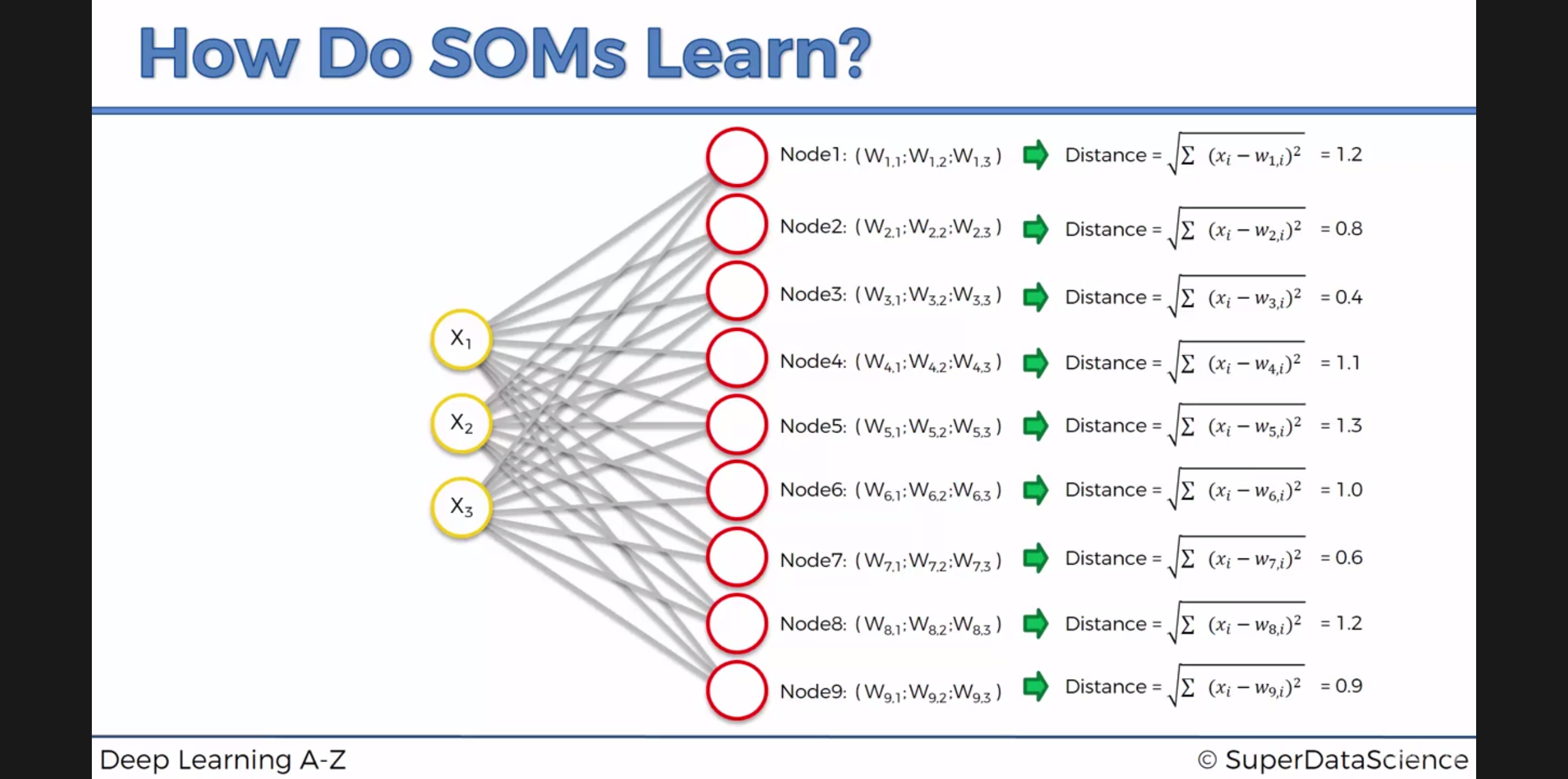
3*3 사이즈의 map 은 9개의 map point = Node 로 이루어졍있고, 각 Node 는 데이터의 차원수와 동일한 parameter 갯수를 가집니다.
사진에서는 3차원 X(x1,x2,x3) 데이터 이므로 Node_i(w_i1, w_i2, w_i3) 가 i=1~9 로 존재합니다.
이제 이 각각의 Node 들과 각 데이터 X 사이의 거리를 구합니다.
이들중 데이터와 가장 가까운 node 를 winning node 라고 마킹합니다.
점(w1i,w2i,w3i)들과 데이터의 feature인 (x1,x2,x3) 점과의 distance 를 좁혀나갑니다.
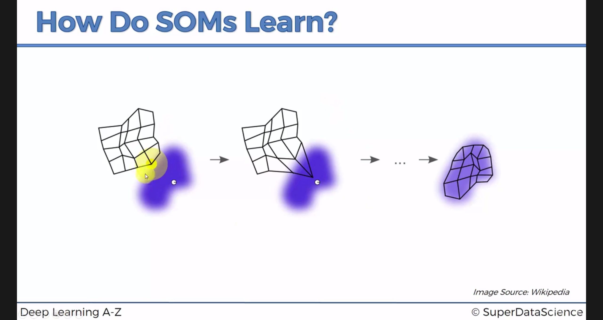
아래는 map 을 데이터에 맞게 점점 fitting 시키는 모습입니다.
특정 데이터 점 하나가 SOMap 의 한 점을 점점 끌어당기는 모습입니다.
(실제론 winning node 와 그 주변 node 까지 동시에 끌어당깁니다.)
이런식으로 모든 데이터에 대해 SOMap 의 각 점을 끌어오면 SOMap 완성됩니다.
SOM의 특징
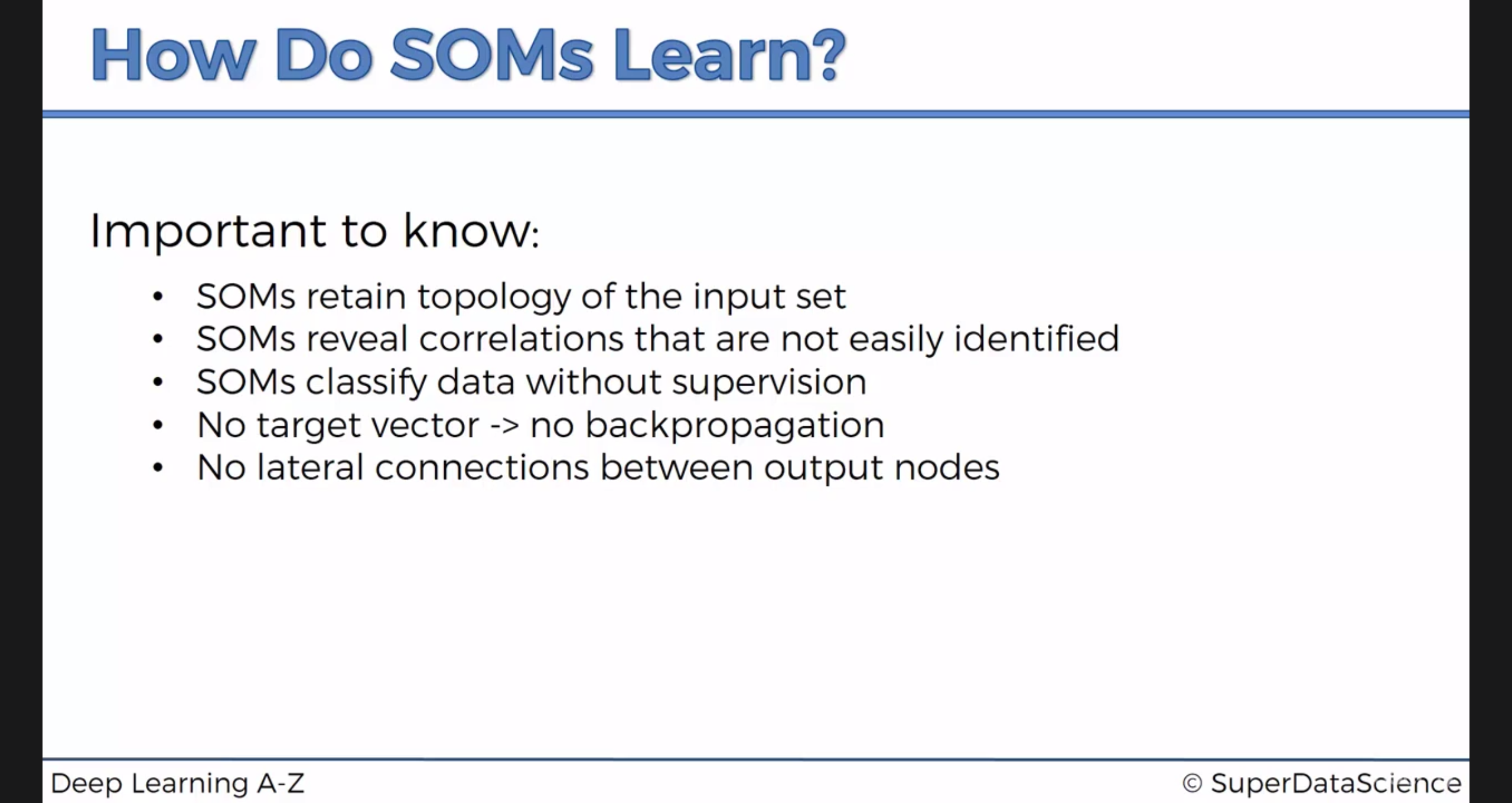
SOM 의 특징은 아래와 같습니다.
- SOM 은 Input 데이터들 사이의 위상을 잘 나타냅니다.
- SOM 은 잘 구별되지 않는 데이터간의 correlation 을 찾아낼 수 있습니다.
- SOM 은 비지도 학습으로 Clustering 을 수행할 수 있습니다.
- 비지도이고, Label Data 가 없으므로, Back propagation 과정도 없습니다.
- output node 간에 후속 연결이 없습니다.
Training 전략
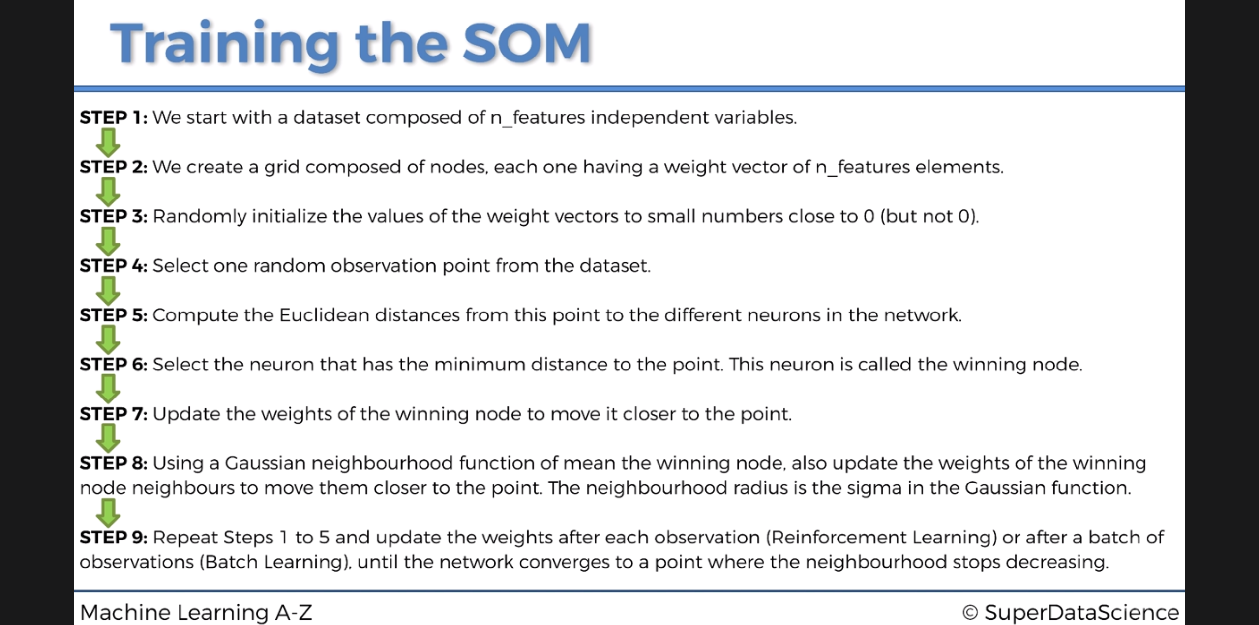
자세한 SOM 의 학습 과정은 아래와 같습니다.
Python Code
- SOM model code
- SOM model use code
1. SOM model code
from math import sqrt

from numpy import (array, unravel_index, nditer, linalg, random, subtract,
                   power, exp, pi, zeros, arange, outer, meshgrid, dot)
from collections import defaultdict
from warnings import warn


"""
    Minimalistic implementation of the Self Organizing Maps (SOM).
"""


def fast_norm(x):
    """Returns norm-2 of a 1-D numpy array.

    * faster than linalg.norm in case of 1-D arrays (numpy 1.9.2rc1).
    """
    return sqrt(dot(x, x.T))


class MiniSom(object):
    def __init__(self, x, y, input_len, sigma=1.0, learning_rate=0.5, decay_function=None, random_seed=None):
        """
            Initializes a Self Organizing Maps.

            x,y - dimensions of the SOM

            input_len - number of the elements of the vectors in input

            sigma - spread of the neighborhood function (Gaussian), needs to be adequate to the dimensions of the map.
            (at the iteration t we have sigma(t) = sigma / (1 + t/T) where T is #num_iteration/2)

            learning_rate - initial learning rate
            (at the iteration t we have learning_rate(t) = learning_rate / (1 + t/T) where T is #num_iteration/2)

            decay_function, function that reduces learning_rate and sigma at each iteration
                            default function: lambda x,current_iteration,max_iter: x/(1+current_iteration/max_iter)

            random_seed, random seed to use.
        """
        if sigma >= x/2.0 or sigma >= y/2.0:
            warn('Warning: sigma is too high for the dimension of the map.')
        if random_seed:
            self.random_generator = random.RandomState(random_seed)
        else:
            self.random_generator = random.RandomState(random_seed)
        if decay_function:
            self._decay_function = decay_function
        else:
            self._decay_function = lambda x, t, max_iter: x/(1+t/max_iter)
        self.learning_rate = learning_rate
        self.sigma = sigma
        self.weights = self.random_generator.rand(x,y,input_len)*2-1 # random initialization
        for i in range(x):
            for j in range(y):
                self.weights[i,j] = self.weights[i,j] / fast_norm(self.weights[i,j]) # normalization
        self.activation_map = zeros((x,y))
        self.neigx = arange(x)
        self.neigy = arange(y) # used to evaluate the neighborhood function
        self.neighborhood = self.gaussian

    def _activate(self, x):
        """ Updates matrix activation_map, in this matrix the element i,j is the response of the neuron i,j to x """
        s = subtract(x, self.weights) # x - w
        it = nditer(self.activation_map, flags=['multi_index'])
        while not it.finished:
            self.activation_map[it.multi_index] = fast_norm(s[it.multi_index])  # || x - w ||
            it.iternext()

    def activate(self, x):
        """ Returns the activation map to x """
        self._activate(x)
        return self.activation_map

    def gaussian(self, c, sigma):
        """ Returns a Gaussian centered in c """
        d = 2*pi*sigma*sigma
        ax = exp(-power(self.neigx-c[0], 2)/d)
        ay = exp(-power(self.neigy-c[1], 2)/d)
        return outer(ax, ay)  # the external product gives a matrix

    def diff_gaussian(self, c, sigma):
        """ Mexican hat centered in c (unused) """
        xx, yy = meshgrid(self.neigx, self.neigy)
        p = power(xx-c[0], 2) + power(yy-c[1], 2)
        d = 2*pi*sigma*sigma
        return exp(-p/d)*(1-2/d*p)

    def winner(self, x):
        """ Computes the coordinates of the winning neuron for the sample x """
        self._activate(x)
        return unravel_index(self.activation_map.argmin(), self.activation_map.shape)

    def update(self, x, win, t):
        """
            Updates the weights of the neurons.
            x - current pattern to learn
            win - position of the winning neuron for x (array or tuple).
            t - iteration index
        """
        eta = self._decay_function(self.learning_rate, t, self.T)
        sig = self._decay_function(self.sigma, t, self.T) # sigma and learning rate decrease with the same rule
        g = self.neighborhood(win, sig)*eta # improves the performances
        it = nditer(g, flags=['multi_index'])
        while not it.finished:
            # eta * neighborhood_function * (x-w)
            self.weights[it.multi_index] += g[it.multi_index]*(x-self.weights[it.multi_index])
            # normalization
            self.weights[it.multi_index] = self.weights[it.multi_index] / fast_norm(self.weights[it.multi_index])
            it.iternext()

    def quantization(self, data):
        """ Assigns a code book (weights vector of the winning neuron) to each sample in data. """
        q = zeros(data.shape)
        for i, x in enumerate(data):
            q[i] = self.weights[self.winner(x)]
        return q

    def random_weights_init(self, data):
        """ Initializes the weights of the SOM picking random samples from data """
        it = nditer(self.activation_map, flags=['multi_index'])
        while not it.finished:
            self.weights[it.multi_index] = data[self.random_generator.randint(len(data))]
            self.weights[it.multi_index] = self.weights[it.multi_index]/fast_norm(self.weights[it.multi_index])
            it.iternext()

    def train_random(self, data, num_iteration):
        """ Trains the SOM picking samples at random from data """
        self._init_T(num_iteration)
        for iteration in range(num_iteration):
            rand_i = self.random_generator.randint(len(data)) # pick a random sample
            self.update(data[rand_i], self.winner(data[rand_i]), iteration)

    def train_batch(self, data, num_iteration):
        """ Trains using all the vectors in data sequentially """
        self._init_T(len(data)*num_iteration)
        iteration = 0
        while iteration < num_iteration:
            idx = iteration % (len(data)-1)
            self.update(data[idx], self.winner(data[idx]), iteration)
            iteration += 1

    def _init_T(self, num_iteration):
        """ Initializes the parameter T needed to adjust the learning rate """
        self.T = num_iteration/2  # keeps the learning rate nearly constant for the last half of the iterations

    def distance_map(self):
        """ Returns the distance map of the weights.
            Each cell is the normalised sum of the distances between a neuron and its neighbours.
        """
        um = zeros((self.weights.shape[0], self.weights.shape[1]))
        it = nditer(um, flags=['multi_index'])
        while not it.finished:
            for ii in range(it.multi_index[0]-1, it.multi_index[0]+2):
                for jj in range(it.multi_index[1]-1, it.multi_index[1]+2):
                    if ii >= 0 and ii < self.weights.shape[0] and jj >= 0 and jj < self.weights.shape[1]:
                        um[it.multi_index] += fast_norm(self.weights[ii, jj, :]-self.weights[it.multi_index])
            it.iternext()
        um = um/um.max()
        return um

    def activation_response(self, data):
        """
            Returns a matrix where the element i,j is the number of times
            that the neuron i,j have been winner.
        """
        a = zeros((self.weights.shape[0], self.weights.shape[1]))
        for x in data:
            a[self.winner(x)] += 1
        return a

    def quantization_error(self, data):
        """
            Returns the quantization error computed as the average distance between
            each input sample and its best matching unit.
        """
        error = 0
        for x in data:
            error += fast_norm(x-self.weights[self.winner(x)])
        return error/len(data)

    def win_map(self, data):
        """
            Returns a dictionary wm where wm[(i,j)] is a list with all the patterns
            that have been mapped in the position i,j.
        """
        winmap = defaultdict(list)
        for x in data:
            winmap[self.winner(x)].append(x)
        return winmap

### unit tests
'''
from numpy.testing import assert_almost_equal, assert_array_almost_equal, assert_array_equal


class TestMinisom:
    def setup_method(self, method):
        self.som = MiniSom(5, 5, 1)
        for i in range(5):
            for j in range(5):
                assert_almost_equal(1.0, linalg.norm(self.som.weights[i,j]))  # checking weights normalization
        self.som.weights = zeros((5, 5))  # fake weights
        self.som.weights[2, 3] = 5.0
        self.som.weights[1, 1] = 2.0

    def test_decay_function(self):
        assert self.som._decay_function(1., 2., 3.) == 1./(1.+2./3.)

    def test_fast_norm(self):
        assert fast_norm(array([1, 3])) == sqrt(1+9)

    def test_gaussian(self):
        bell = self.som.gaussian((2, 2), 1)
        assert bell.max() == 1.0
        assert bell.argmax() == 12  # unravel(12) = (2,2)

    def test_win_map(self):
        winners = self.som.win_map([5.0, 2.0])
        assert winners[(2, 3)][0] == 5.0
        assert winners[(1, 1)][0] == 2.0

    def test_activation_reponse(self):
        response = self.som.activation_response([5.0, 2.0])
        assert response[2, 3] == 1
        assert response[1, 1] == 1

    def test_activate(self):
        assert self.som.activate(5.0).argmin() == 13.0  # unravel(13) = (2,3)

    def test_quantization_error(self):
        self.som.quantization_error([5, 2]) == 0.0
        self.som.quantization_error([4, 1]) == 0.5

    def test_quantization(self):
        q = self.som.quantization(array([4, 2]))
        assert q[0] == 5.0
        assert q[1] == 2.0

    def test_random_seed(self):
        som1 = MiniSom(5, 5, 2, sigma=1.0, learning_rate=0.5, random_seed=1)
        som2 = MiniSom(5, 5, 2, sigma=1.0, learning_rate=0.5, random_seed=1)
        assert_array_almost_equal(som1.weights, som2.weights)  # same initialization
        data = random.rand(100,2)
        som1 = MiniSom(5, 5, 2, sigma=1.0, learning_rate=0.5, random_seed=1)
        som1.train_random(data,10)
        som2 = MiniSom(5, 5, 2, sigma=1.0, learning_rate=0.5, random_seed=1)
        som2.train_random(data,10)
        assert_array_almost_equal(som1.weights,som2.weights)  # same state after training

    def test_train_batch(self):
        som = MiniSom(5, 5, 2, sigma=1.0, learning_rate=0.5, random_seed=1)
        data = array([[4, 2], [3, 1]])
        q1 = som.quantization_error(data)
        som.train_batch(data, 10)
        assert q1 > som.quantization_error(data)

    def test_train_random(self):
        som = MiniSom(5, 5, 2, sigma=1.0, learning_rate=0.5, random_seed=1)
        data = array([[4, 2], [3, 1]])
        q1 = som.quantization_error(data)
        som.train_random(data, 10)
        assert q1 > som.quantization_error(data)

    def test_random_weights_init(self):
        som = MiniSom(2, 2, 2, random_seed=1)
        som.random_weights_init(array([[1.0, .0]]))
        for w in som.weights:
            assert_array_equal(w[0], array([1.0, .0]))


'''
2. SOM model use code
만든 SOM model 을 이용해 Credit card 발급 신청자 데이터를 Clustering 해보고, 수상한 사람을 찾아내보도록 하겠습니다.
우선 데이터를 불러옵니다.
import numpy as np
import matplotlib.pyplot as plt
import pandas as pd
%matplotlib inline
#Importing the dataset
dataset = pd.read_csv('Credit_Card_Applications.csv')
X = dataset.iloc[:, :-1].values
y = dataset.iloc[:, -1].values
dataset
| CustomerID | A1 | A2 | A3 | A4 | A5 | A6 | A7 | A8 | A9 | A10 | A11 | A12 | A13 | A14 | Class | |
|---|---|---|---|---|---|---|---|---|---|---|---|---|---|---|---|---|
| 0 | 15776156 | 1 | 22.08 | 11.460 | 2 | 4 | 4 | 1.585 | 0 | 0 | 0 | 1 | 2 | 100 | 1213 | 0 |
| 1 | 15739548 | 0 | 22.67 | 7.000 | 2 | 8 | 4 | 0.165 | 0 | 0 | 0 | 0 | 2 | 160 | 1 | 0 |
| 2 | 15662854 | 0 | 29.58 | 1.750 | 1 | 4 | 4 | 1.250 | 0 | 0 | 0 | 1 | 2 | 280 | 1 | 0 |
| 3 | 15687688 | 0 | 21.67 | 11.500 | 1 | 5 | 3 | 0.000 | 1 | 1 | 11 | 1 | 2 | 0 | 1 | 1 |
| 4 | 15715750 | 1 | 20.17 | 8.170 | 2 | 6 | 4 | 1.960 | 1 | 1 | 14 | 0 | 2 | 60 | 159 | 1 |
| 5 | 15571121 | 0 | 15.83 | 0.585 | 2 | 8 | 8 | 1.500 | 1 | 1 | 2 | 0 | 2 | 100 | 1 | 1 |
| 6 | 15726466 | 1 | 17.42 | 6.500 | 2 | 3 | 4 | 0.125 | 0 | 0 | 0 | 0 | 2 | 60 | 101 | 0 |
| 7 | 15660390 | 0 | 58.67 | 4.460 | 2 | 11 | 8 | 3.040 | 1 | 1 | 6 | 0 | 2 | 43 | 561 | 1 |
| 8 | 15663942 | 1 | 27.83 | 1.000 | 1 | 2 | 8 | 3.000 | 0 | 0 | 0 | 0 | 2 | 176 | 538 | 0 |
| 9 | 15638610 | 0 | 55.75 | 7.080 | 2 | 4 | 8 | 6.750 | 1 | 1 | 3 | 1 | 2 | 100 | 51 | 0 |
| 10 | 15644446 | 1 | 33.50 | 1.750 | 2 | 14 | 8 | 4.500 | 1 | 1 | 4 | 1 | 2 | 253 | 858 | 1 |
| 11 | 15585892 | 1 | 41.42 | 5.000 | 2 | 11 | 8 | 5.000 | 1 | 1 | 6 | 1 | 2 | 470 | 1 | 1 |
| 12 | 15609356 | 1 | 20.67 | 1.250 | 1 | 8 | 8 | 1.375 | 1 | 1 | 3 | 1 | 2 | 140 | 211 | 0 |
| 13 | 15803378 | 1 | 34.92 | 5.000 | 2 | 14 | 8 | 7.500 | 1 | 1 | 6 | 1 | 2 | 0 | 1001 | 1 |
| 14 | 15599440 | 1 | 58.58 | 2.710 | 2 | 8 | 4 | 2.415 | 0 | 0 | 0 | 1 | 2 | 320 | 1 | 0 |
| 15 | 15692408 | 1 | 48.08 | 6.040 | 2 | 4 | 4 | 0.040 | 0 | 0 | 0 | 0 | 2 | 0 | 2691 | 1 |
| 16 | 15683168 | 1 | 29.58 | 4.500 | 2 | 9 | 4 | 7.500 | 1 | 1 | 2 | 1 | 2 | 330 | 1 | 1 |
| 17 | 15790254 | 0 | 18.92 | 9.000 | 2 | 6 | 4 | 0.750 | 1 | 1 | 2 | 0 | 2 | 88 | 592 | 1 |
| 18 | 15767729 | 1 | 20.00 | 1.250 | 1 | 4 | 4 | 0.125 | 0 | 0 | 0 | 0 | 2 | 140 | 5 | 0 |
| 19 | 15768600 | 0 | 22.42 | 5.665 | 2 | 11 | 4 | 2.585 | 1 | 1 | 7 | 0 | 2 | 129 | 3258 | 1 |
| 20 | 15699839 | 0 | 28.17 | 0.585 | 2 | 6 | 4 | 0.040 | 0 | 0 | 0 | 0 | 2 | 260 | 1005 | 0 |
| 21 | 15786237 | 0 | 19.17 | 0.585 | 1 | 6 | 4 | 0.585 | 1 | 0 | 0 | 1 | 2 | 160 | 1 | 0 |
| 22 | 15694530 | 1 | 41.17 | 1.335 | 2 | 2 | 4 | 0.165 | 0 | 0 | 0 | 0 | 2 | 168 | 1 | 0 |
| 23 | 15796813 | 1 | 41.58 | 1.750 | 2 | 4 | 4 | 0.210 | 1 | 0 | 0 | 0 | 2 | 160 | 1 | 0 |
| 24 | 15605791 | 1 | 19.50 | 9.585 | 2 | 6 | 4 | 0.790 | 0 | 0 | 0 | 0 | 2 | 80 | 351 | 0 |
| 25 | 15714087 | 1 | 32.75 | 1.500 | 2 | 13 | 8 | 5.500 | 1 | 1 | 3 | 1 | 2 | 0 | 1 | 1 |
| 26 | 15711446 | 1 | 22.50 | 0.125 | 1 | 4 | 4 | 0.125 | 0 | 0 | 0 | 0 | 2 | 200 | 71 | 0 |
| 27 | 15588123 | 1 | 33.17 | 3.040 | 1 | 8 | 8 | 2.040 | 1 | 1 | 1 | 1 | 2 | 180 | 18028 | 1 |
| 28 | 15748552 | 0 | 30.67 | 12.000 | 2 | 8 | 4 | 2.000 | 1 | 1 | 1 | 0 | 2 | 220 | 20 | 1 |
| 29 | 15618410 | 1 | 23.08 | 2.500 | 2 | 8 | 4 | 1.085 | 1 | 1 | 11 | 1 | 2 | 60 | 2185 | 1 |
| ... | ... | ... | ... | ... | ... | ... | ... | ... | ... | ... | ... | ... | ... | ... | ... | ... |
| 660 | 15598586 | 1 | 26.67 | 2.710 | 1 | 13 | 4 | 5.250 | 1 | 1 | 1 | 0 | 2 | 211 | 1 | 1 |
| 661 | 15665014 | 0 | 22.50 | 0.415 | 2 | 3 | 4 | 0.335 | 0 | 0 | 0 | 1 | 1 | 144 | 1 | 0 |
| 662 | 15701738 | 1 | 39.92 | 0.540 | 1 | 6 | 4 | 0.500 | 1 | 1 | 3 | 0 | 2 | 200 | 1001 | 1 |
| 663 | 15650591 | 0 | 26.08 | 8.665 | 2 | 6 | 4 | 1.415 | 1 | 0 | 0 | 0 | 2 | 160 | 151 | 1 |
| 664 | 15652667 | 1 | 20.00 | 0.000 | 2 | 2 | 4 | 0.500 | 0 | 0 | 0 | 0 | 2 | 144 | 1 | 0 |
| 665 | 15679622 | 1 | 31.57 | 4.000 | 1 | 3 | 4 | 0.085 | 0 | 0 | 0 | 1 | 2 | 411 | 1 | 0 |
| 666 | 15730150 | 1 | 26.75 | 4.500 | 1 | 8 | 5 | 2.500 | 0 | 0 | 0 | 0 | 2 | 200 | 1211 | 0 |
| 667 | 15813192 | 0 | 24.92 | 1.250 | 2 | 1 | 1 | 0.000 | 1 | 0 | 0 | 0 | 2 | 80 | 1 | 0 |
| 668 | 15606554 | 0 | 32.25 | 1.500 | 2 | 8 | 4 | 0.250 | 0 | 0 | 0 | 1 | 2 | 372 | 123 | 0 |
| 669 | 15611794 | 1 | 17.67 | 4.460 | 2 | 8 | 4 | 0.250 | 0 | 0 | 0 | 0 | 1 | 80 | 1 | 0 |
| 670 | 15672357 | 0 | 37.75 | 5.500 | 2 | 11 | 4 | 0.125 | 1 | 0 | 0 | 1 | 2 | 228 | 1 | 1 |
| 671 | 15711759 | 1 | 22.67 | 2.540 | 1 | 8 | 8 | 2.585 | 1 | 0 | 0 | 0 | 2 | 0 | 1 | 1 |
| 672 | 15615296 | 0 | 17.92 | 10.210 | 2 | 1 | 1 | 0.000 | 0 | 0 | 0 | 0 | 2 | 0 | 51 | 0 |
| 673 | 15699294 | 1 | 24.42 | 12.335 | 2 | 11 | 8 | 1.585 | 1 | 0 | 0 | 1 | 2 | 120 | 1 | 1 |
| 674 | 15788634 | 0 | 25.75 | 0.500 | 2 | 8 | 8 | 0.875 | 1 | 0 | 0 | 1 | 2 | 491 | 1 | 1 |
| 675 | 15660871 | 1 | 26.17 | 12.500 | 1 | 4 | 8 | 1.250 | 0 | 0 | 0 | 1 | 2 | 0 | 18 | 0 |
| 676 | 15618258 | 0 | 22.75 | 6.165 | 2 | 6 | 4 | 0.165 | 0 | 0 | 0 | 0 | 2 | 220 | 1001 | 0 |
| 677 | 15722535 | 1 | 23.00 | 0.750 | 2 | 7 | 4 | 0.500 | 1 | 0 | 0 | 1 | 1 | 320 | 1 | 0 |
| 678 | 15711977 | 1 | 25.67 | 0.290 | 1 | 8 | 4 | 1.500 | 0 | 0 | 0 | 1 | 2 | 160 | 1 | 0 |
| 679 | 15690169 | 1 | 48.58 | 0.205 | 1 | 4 | 4 | 0.250 | 1 | 1 | 11 | 0 | 2 | 380 | 2733 | 1 |
| 680 | 15790689 | 1 | 21.17 | 0.000 | 2 | 8 | 4 | 0.500 | 0 | 0 | 0 | 1 | 1 | 0 | 1 | 0 |
| 681 | 15665181 | 1 | 35.25 | 16.500 | 1 | 8 | 4 | 4.000 | 1 | 0 | 0 | 0 | 2 | 80 | 1 | 0 |
| 682 | 15633608 | 0 | 22.92 | 11.585 | 2 | 13 | 4 | 0.040 | 1 | 0 | 0 | 0 | 2 | 80 | 1350 | 1 |
| 683 | 15805261 | 0 | 48.17 | 1.335 | 2 | 3 | 7 | 0.335 | 0 | 0 | 0 | 0 | 2 | 0 | 121 | 0 |
| 684 | 15740356 | 1 | 43.00 | 0.290 | 1 | 13 | 8 | 1.750 | 1 | 1 | 8 | 0 | 2 | 100 | 376 | 1 |
| 685 | 15808223 | 1 | 31.57 | 10.500 | 2 | 14 | 4 | 6.500 | 1 | 0 | 0 | 0 | 2 | 0 | 1 | 1 |
| 686 | 15769980 | 1 | 20.67 | 0.415 | 2 | 8 | 4 | 0.125 | 0 | 0 | 0 | 0 | 2 | 0 | 45 | 0 |
| 687 | 15675450 | 0 | 18.83 | 9.540 | 2 | 6 | 4 | 0.085 | 1 | 0 | 0 | 0 | 2 | 100 | 1 | 1 |
| 688 | 15776494 | 0 | 27.42 | 14.500 | 2 | 14 | 8 | 3.085 | 1 | 1 | 1 | 0 | 2 | 120 | 12 | 1 |
| 689 | 15592412 | 1 | 41.00 | 0.040 | 2 | 10 | 4 | 0.040 | 0 | 1 | 1 | 0 | 1 | 560 | 1 | 1 |
690 rows × 16 columns
데이터를 보시면 첫번째줄은 고객 식별번호id 이고 마지막줄은 카드발급 승인 여부입니다.
이중 마지막 카드발급 승인여부는 따로 y 로 빼둡니다.
Clustering 에 고려할 feature 가 아니기 때문입니다. 그리고 나중에 Clustering 이 잘 되었는지 확인해 볼 때 사용합니다.
데이터를 Min=0, Max=1 이 되도록 Scaling 해줍니다.
불필요한 연산량을 줄이는데 도움됩니다.
sklearn 의 preprocessing 모듈을 이용하면 편리하게 scaling 작업을 하실 수 있습니다.
# Feature Scaling
from sklearn.preprocessing import MinMaxScaler
sc = MinMaxScaler(feature_range = (0, 1))
X = sc.fit_transform(X)
plt.plot(X[:,2]) #checking the scaling result of A2
[<matplotlib.lines.Line2D at 0x11775c048>]

그래프를 보시면 0과 1사이의 값으로 잘 Scaling 된것을 보실 수 있습니다.
이제 데이터 준비가 완료되었으니, 준비된 데이터들을 clustering 해봅시다.
# Training the SOM
#from minisom import MiniSom
som = MiniSom(x = 10, y = 10, input_len = 15, sigma = 1.0, learning_rate = 0.5)
som.random_weights_init(X)
som.train_random(data = X, num_iteration = 100)
만들어놓은 MiniSom model 을 불러오고 Default map 사이즈와 input dimension을 지정해줍니다.
random_weight_init 으로 각 node 들을 초기화시켜준 후
train_random 메서드로 SOM 학습을 시작합니다.
3. 확인
학습이 끝나고 학습의 결과를 pylab 모듈을 통해 확인하겠습니다.
우선 10*10 map 을 평면 위에 표현하고
node 에 최근접한 data point 들이 많을수록 짙게, 적을수록 옅게 표시해줍니다.
Map 의 진한 부분엔 데이터들이 모여있다는 뜻입니다. (Clustering 된것입니다.)
따로 빼놓은 y : 카드 발급 여부 데이터를 이제 사용합니다.
Map 위에 data point 들에 대응되는 y 를 표현합니다.
data point 와 최근접한 node 위에 data point가 발급 승인된 고객이면 초록네모, 발급 거절된 고객이면 빨간동그라미로 마킹합니다.
진한 node 위에 마킹이 많이 될 것입니다.
# Visualizing the results
from pylab import bone, pcolor, colorbar, plot, show
bone()
pcolor(som.distance_map().T)
colorbar()
markers = ['o', 's']
colors = ['r', 'g']
for i, x in enumerate(X):
    w = som.winner(x)
    plot(w[0] + 0.5,
         w[1] + 0.5,
         markers[y[i]],
         markeredgecolor = colors[y[i]],
         markerfacecolor = 'None',
         markersize = 10,
         markeredgewidth = 2)
show()

이제 결과를 보시면, Map의 진한부분은 데이터가 많이 모인부분, 연한부분은 데이터가 거의 없는 부분이라고 보시면 되는데
이상한 점은 node 가 하얗게 표시된, 연결된 데이터포인트가 거의 없는, 즉 응집이 전혀 없는 부분에 존재하는 데이터들입니다.
저 고객들은 다른 고객들과 전혀 다른 feature 의 구성을 띄고 있어서, 어느 cluster 에도 끼지 못했습니다.
저런 고객들은 수상하죠. 잠재 위험 고객으로 분류합니다.
# Finding the frauds
mappings = som.win_map(X)
frauds = np.concatenate((mappings[(1,4)], mappings[(2,9)]), axis = 0)
frauds = sc.inverse_transform(frauds)
frauds.shape #수상한 data 56개 : 다른 데이터들과 거리가 멀다
(56, 15)
수상한 데이터 56개가 검출되었습니다.
아래를 보시면 node(1,4) 에 38개가 수상하고, node(2,9)에 18개가 수상합니다.
np.array(mappings[(1,4)]).shape #(1,4) node 가 winning node(가장가까운노드) 인 data의 갯수 : 38개
(38, 15)
np.array(mappings[(2,9)]).shape #(2,9) node 가 winning node(가장가까운노드) 인 data의 갯수 : 18개
(18, 15)
수상한 고객들의 id 를 뽑아서 확인해보겠습니다.
frauds_customers_id=frauds[:, 0]
frauds_customers_id
array([ 15739548.,  15699839.,  15648069.,  15731586.,  15705918.,
        15706762.,  15672894.,  15575605.,  15644453.,  15783883.,
        15756538.,  15694666.,  15728523.,  15646594.,  15593959.,
        15629750.,  15675926.,  15794204.,  15734008.,  15592999.,
        15757434.,  15769548.,  15742009.,  15593834.,  15673907.,
        15737909.,  15599272.,  15660528.,  15779207.,  15711299.,
        15609987.,  15752578.,  15721504.,  15666096.,  15609758.,
        15611682.,  15618258.,  15805261.,  15767729.,  15711446.,
        15720529.,  15787693.,  15688210.,  15704509.,  15793366.,
        15793317.,  15735106.,  15688059.,  15646521.,  15683276.,
        15652289.,  15768777.,  15791326.,  15678779.,  15779586.,
        15730150.])
마치며
이렇게 SOM 을 간단하게 살펴보았습니다.
궁금한 점 댓글로 남겨주시기 바랍니다. 감사합니다^^.